
In the last post we introduced the need for quantum mechanics in thinking about the classical model of atoms. A whole undergraduate course is needed to properly define and derive the implications of QM. In fact at CMU we actually give physics majors two and a half semesters of QM. Here we will jump straight to the upshot.
QM tells us that we shouldn’t talk about the trajectories of the electron within an atom. We shouldn’t talk about where the electron is within the atom at a certain time, what is its path and how is it accelerating, like you would do in Newton’s physics (or in Einstein’s relativity). Instead, there is a new mathematical concept called the “Amplitude”, often written as ψ, which is really the fundamental physical entity. It’s the thing that describes everything there is to know about the electron. Everything we see in nature is encoded in the amplitude.
The theory of Quantum Mechanics tells us how the amplitude changes in time and gives us a prescription for translating from the amplitude to concrete physical questions that we might want to ask. QM tells us that amplitudes evolve in time like waves. It also provides a way to convert these amplitudes into probabilities (more on this below).
You can see already that the character of this revolution is much different than relativity. In relativity, we still had these intuitive physical notions of speed, trajectories, etc. QM is much more abstract, much more formal. There is this completely new abstract entity that we have to track in order to describe reality.
QM is also, in almost all cases, much less predictive than Newtonian physics. Instead of telling us what happens, it tells us what the probability is for certain things to happen. QM tells us there is a fundamental, inherent randomness in nature. In Newton’s physics, if you knew the positions and momenta of all the particles at a given time, you could predict with certainty what is going to happen at all later times. Nature, in this picture, is deterministic. QM throws this out the window.
Here is an example using muons, a particle we talked about already in the context of relativity. We can create two muons that have exactly the same amplitude.
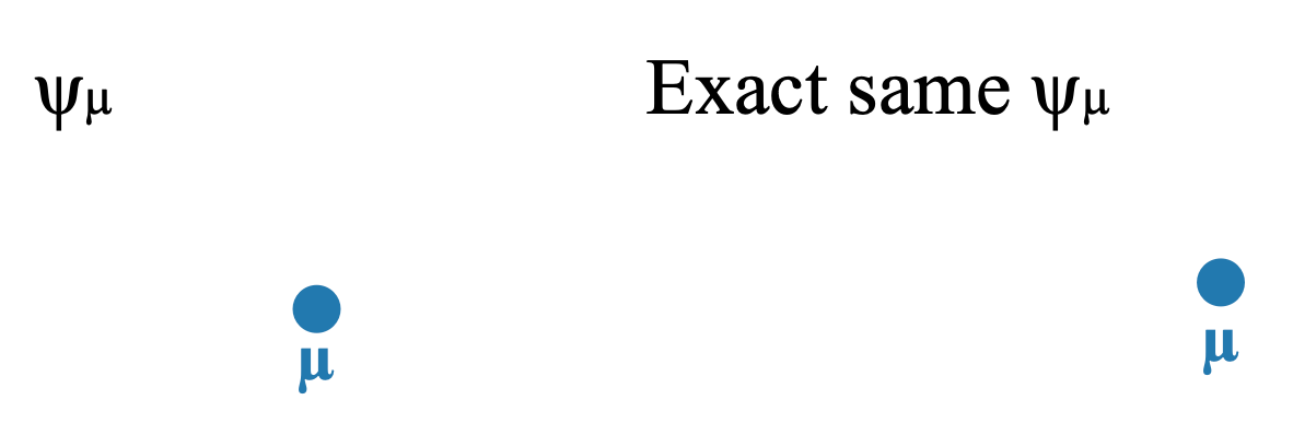
We noted before that muons have a finite lifetime, they decay into other particles after a characteristic time. When the muons decay they turn into an electron, a neutrino, and an anti-neutrino1.
If we watch our two muons, we might find that one of the muons decays after 2.1 microseconds with a particular angle θ between the electron and anti-neutrino, whereas the other decays after 2.3 microseconds, with a different angle among its decay products.
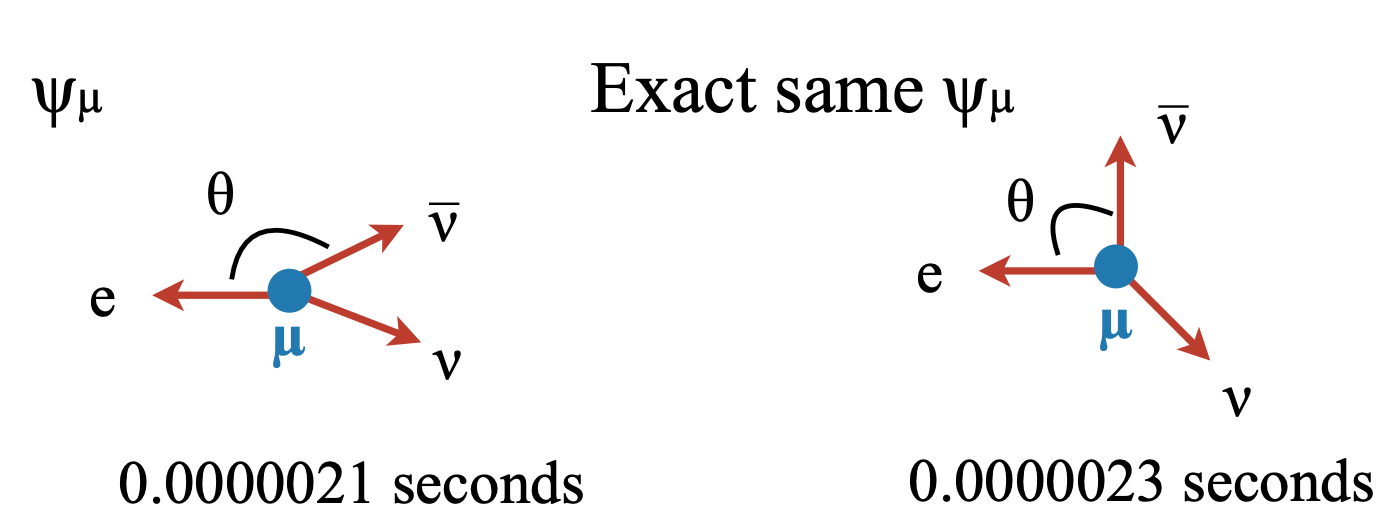
Now remember the amplitude contains everything there is to know about the particles. In terms of the theory these two particles are exactly identical. In QM identical initial states can lead to different outcomes. QM cannot predict what is going to happen in any particular event. In our example, it can’t tell us exactly how long the first muon will live and what its decay angle will be.
What QM can predict is the distributions of outcomes of many identically prepared initial states, ie: the relative probability of seeing a muon live a certain amount of time and decay with a particular angle. The amplitude encodes the probability distribution; QM tells us that the probability is given by the square of the amplitude.
Next time we will discuss another major outcome of QM: the uncertainty principle.
We will talk more about neutrinos and anti-particles later in the series.